import numpy as np
import matplotlib.pyplot as plt
import matplotlib as mpl
import sympy as sy
import statsmodels.api as sm

from sympy import init_printing

init_printing()

plt.style.use("ggplot")

This chapter focuses on the features of sampling distribution of OLS estimator. We would like to know that if OLS can provide us with unbiased, consistent and efficient estimates.

Unbaisedness of OLS

In this chapter, we assume regression model has the form

\[ \boldsymbol{y} = \boldsymbol{X\beta} +\boldsymbol{u}, \quad \boldsymbol{u}\sim \text{IID}(\boldsymbol{0},\sigma^2\mathbf{I}) \]

The notation \(\text{IID}\) means identically independent distributed, \(\sigma^2\mathbf{I}\) is the covariance matrix, being a diagonal matrix means regressors are independently distributed. We also assume all diagonal elements are the same, i.e. \(\sigma^2\), which means homoscedasticity.

If an estimator \(\theta\) is unbiased, it should always satisfy the condition

\[ E(\hat{\theta}) -\theta_0 = 0 \]

To show that the OLS estimator is unbiased, we denote \(\boldsymbol{\beta}_0\) as the true parameter in the data generating process (DGP), that is to say, we would like to see \(E(\boldsymbol{\hat{\beta}})=\boldsymbol{\beta}_0\).

To show the conditions that makes OLS unbiased, we substitute DGP back in OLS formula

\[\begin{align} \hat{\boldsymbol{\beta}}&= (\boldsymbol{X}^T\boldsymbol{X})^{-1}\boldsymbol{X}^T\boldsymbol{y}\\ &=(\boldsymbol{X}^T\boldsymbol{X})^{-1}\boldsymbol{X}^T(\boldsymbol{X}\boldsymbol{\beta}_0+u)\\ & = \boldsymbol{\beta}_0 + (\boldsymbol{X}^T\boldsymbol{X})^{-1}\boldsymbol{X}^T\boldsymbol{u} \end{align}\]

First, we assume \(\boldsymbol{X}\) to be nonstochastic, also with assumption \(E(\boldsymbol{u}) = 0\), we obtain

\[\begin{align} E(\boldsymbol{\hat{\beta}}) &= \boldsymbol{\beta}_0 + (\boldsymbol{X}^T\boldsymbol{X})^{-1}\boldsymbol{X}^T\boldsymbol{u}\\ &= \boldsymbol{\beta}_0 + (\boldsymbol{X}^T\boldsymbol{X})^{-1}\boldsymbol{X}^TE(\boldsymbol{u})\\ &=\boldsymbol{\beta}_0 \end{align}\] However nonstochastic assumption is limited mostly in cross section data.

Second, we can assume \(\boldsymbol{X}\) exogenous, such that \(E(\boldsymbol{u}|\boldsymbol{X}) = 0\), also proves \(E(\boldsymbol{\hat{\beta}})=\boldsymbol{\beta}_0\). Exogeneity simply means that the randomness of \(\boldsymbol{X}\) has nothing to do with \(\boldsymbol{u}\).

We have even weaker version of exogeneity, \(E(u_t|\boldsymbol{X}_t) = 0\), which excludes the possibility that \(u_t\) might depend on \(X_{t-1}\) or \(X_{t-2}\), etc. It is called predeterminedness condition, which is suitable for time series data.

However, for time series data, OLS shall be used with cautions, it is widely known that OLS is not suitable for \(\text{ARMA}\) model, because \(\boldsymbol{y}\) has lagged dependent variables.

For \(\text{VAR}\), OLS is a common practice, because it doesn’t differentiate endogenous and exogenous variables.

Predetermined Variable vs Exogenous Variable

In strictly speaking, predetermined variables has two categories: exogenous variables and predetermined endogenous variables.

The former one can either be current or lagged, as long as it doesn’t evolve with model’s dynamics. The latter one is common in autoregressive models.

Consistency of OLS

Consistency means the estimates tends to the quantity of true parameters as sample tends to infinity. Now let’s show why OLS estimator is consistent. Start from

\[ \boldsymbol{\hat{\beta}} = \boldsymbol{\beta}_0 + (\boldsymbol{X}^T\boldsymbol{X})^{-1}\boldsymbol{X}^T\boldsymbol{u} \]

We would to like to know if \(\text{plim}\boldsymbol{\hat{\beta}} = \boldsymbol{\beta}_0\), which boils down to verify if

\[ \text{plim}(\boldsymbol{X}^T\boldsymbol{X})^{-1}\boldsymbol{X}^T\boldsymbol{u} =0 \]

However \(\boldsymbol{X}^T\boldsymbol{X}\) and \(\boldsymbol{X}^Tu\) do not have probability limit even if \(n \rightarrow \infty\).

Modify the probability limit we obtain

\[ \bigg(\text{plim}\frac{1}{n}\boldsymbol{X}^T\boldsymbol{X}\bigg)^{-1}\text{plim}\frac{1}{n}\boldsymbol{X}^T\boldsymbol{u} =0 \]

We assume a weaker version of exogeneity \(E(u_t|X_t) = 0\), so is \(E(X_t^Tu_t|X_t)=0\), law of iterated expectation tells that \(E(X_t^Tu_t)=0\). To summarize

\[ \text{plim}\frac{1}{n}\boldsymbol{X}^T\boldsymbol{u}=\text{plim}\frac{1}{n}\sum_{t=1}^nX_t^T u_t = 0 \]

which proves the consistency of OLS.

Simulation of Consistency of OLS

Here we can demonstrate a simple Monte Carlo simulation with true parameters \(\boldsymbol{\beta}_0 = [2, 3, 4, 5]^T\), we increase sample size from \(5\) to \(100\) with a unit increment in each loop, and also with each sample size we redraw the disturbance term \(10\) times, you can experiment with codes below, they might not be concise but considerably intuitive. Pay attention to the plots how they approach the true parameters as sample sizes increase.

sampl_size = np.arange(5, 100)
re_draw = 10

beta_array = np.array([2, 3, 4, 5])
beta_array = beta_array[np.newaxis, :].T

beta_hat_mean = []
for i in sampl_size:
    const = np.ones(i)
    const = const[np.newaxis, :]

    X_inde = np.random.randn(3, i)
    X = np.concatenate((const.T, X_inde.T), axis=1)

    beta_hat = []
    for j in range(re_draw):
        u = np.random.randn(i)
        u = u[np.newaxis, :].T
        y = X @ beta_array + u
        beta_hat.append(np.linalg.inv(X.T @ X) @ X.T @ y)
    beta_hat = np.array(beta_hat).T
    beta_hat_mean.append(np.mean(beta_hat[0], axis=1))

beta0, beta1, beta2, beta3 = [], [], [], []
for i in beta_hat_mean:
    beta0.append(i[0])
    beta1.append(i[1])
    beta2.append(i[2])
    beta3.append(i[3])

fig, ax = plt.subplots(figsize=(18, 8), nrows=2, ncols=2)
fig.suptitle("Simulation of OLS Consistency", size=18)
ax[0, 0].plot(beta0)
ax[0, 0].axhline(2, color="r")
ax[0, 0].set_xlabel(r"$\beta_1$ Sample Size")

ax[0, 1].plot(beta1)
ax[0, 1].axhline(3, color="r")
ax[0, 1].set_xlabel(r"$\beta_2$ Sample Size")

ax[1, 0].plot(beta2)
ax[1, 0].axhline(4, color="r")
ax[1, 0].set_xlabel(r"$\beta_3$ Sample Size")

ax[1, 1].plot(beta3)
ax[1, 1].axhline(5, color="r")
ax[1, 1].set_xlabel(r"$\beta_4$ Sample Size")
plt.show()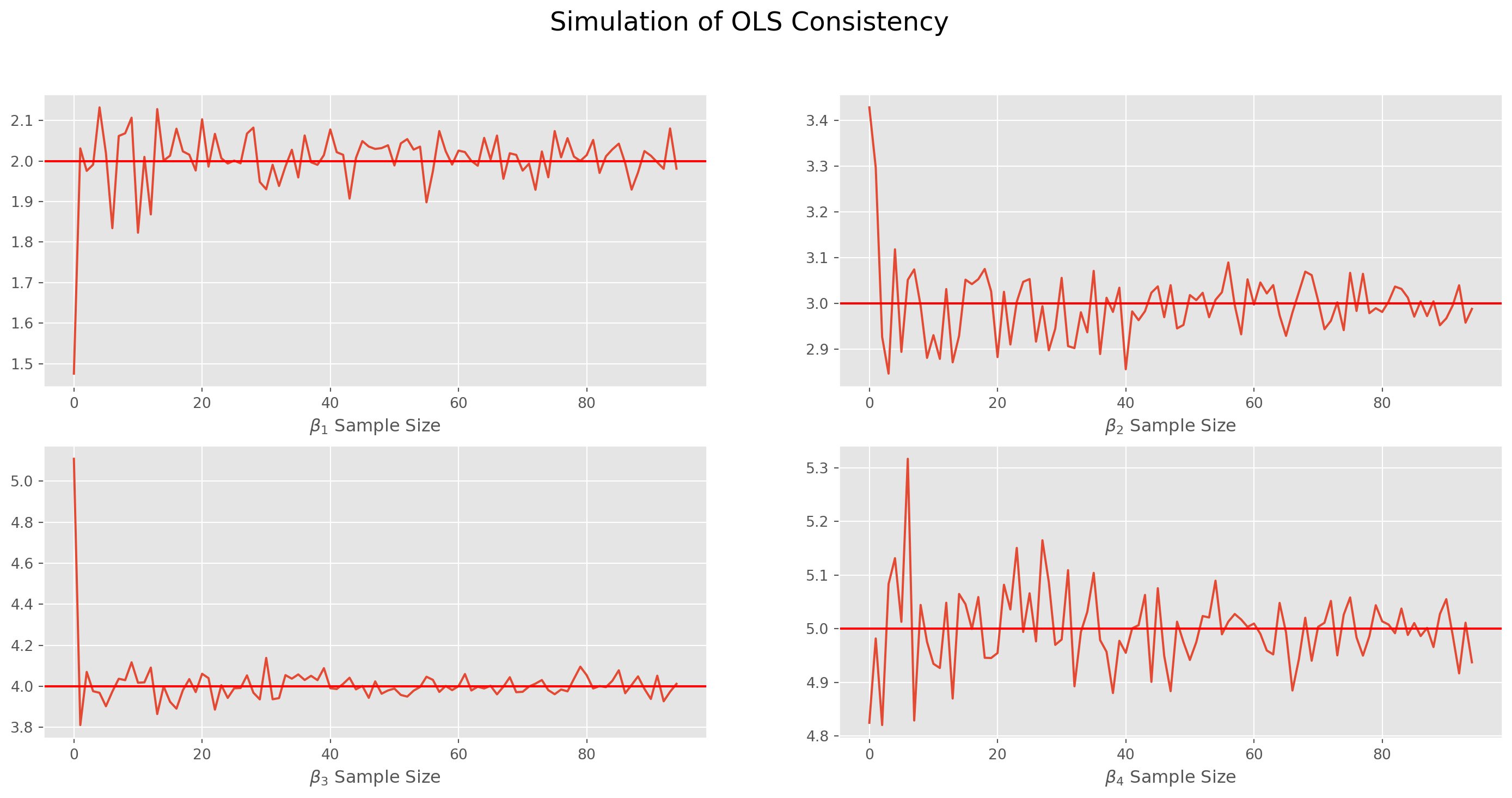

Efficiency of the OLS

The efficiency of estimator represents the capacity of utilizing the information efficiently. For instance, OLS is more efficient than many other estimators, because with the same sample size, OLS yields the estimates with highest precision.

Positive Definite Matrices

Before moving any further, we will refresh the definition of positive definite matrices.

A quadratic form is a function with form \(Q(\mathbf{x})=\mathbf{x}^TA\mathbf{x}\), where \(A\) is an \(n\times n\) symmetric matrix, which is called the the matrix of the quadratic form. For more details, check linear algebra material.

Now some terms to need to be defined, a quadratic form \(Q\) is:

positive definite if \(Q(\mathbf{x})>0\) for all \(\mathbf{x} \neq \mathbf{0}\)
negative definite if \(Q(\mathbf{x})<0\) for all \(\mathbf{x} \neq \mathbf{0}\)
positive semidefinite if \(Q(\mathbf{x})\geq0\) for all \(\mathbf{x} \neq \mathbf{0}\)
negative semidefinite if \(Q(\mathbf{x})\leq0\) for all \(\mathbf{x} \neq \mathbf{0}\)
indefinite if \(Q(\mathbf{x})\) assumes both positive and negative values.

If \(B\) is an \(m\times n\) matrix, both \(B^TB\) and \(BB^T\) yield symmetric matrices. Here is an example of \(B_{3\times 2}\)

B = sy.Matrix([[1, -1], [3, 4], [0, 2]])
B

\(\displaystyle \left[\begin{matrix}1 & -1\\3 & 4\\0 & 2\end{matrix}\right]\)

\(B^TB\) yields a \(2\times2\) matrix

B.T * B

\(\displaystyle \left[\begin{matrix}10 & 11\\11 & 21\end{matrix}\right]\)

\(BB^T\) yields a \(3\times3\) matrix

B * B.T

\(\displaystyle \left[\begin{matrix}2 & -1 & -2\\-1 & 25 & 8\\-2 & 8 & 4\end{matrix}\right]\)

Since \(B^TB\) and \(BB^T\) are both symmetric, \(A\) can be replaced by either of them, technically the Cholesky decomposition can achieve \(A = BB^T\) or \(A = B^TB\).

Actually any matrix of form \(B^TB\) or \(BB^T\) is positive semidefinite, to see this, observe that \[ x^TB^TBx = (Bx)^T(Bx) = \|Bx\|^2 \geq 0\\ xBB^Tx^T = xB (xB)^T = \|xB\|^2\geq 0 \] where \(x\neq0\).

In practice, the second form is quite rare, so we focus the on the first form \(x^TB^TBx\), since \(x\neq 0\), the only condition of \(\|Bx\|^2 = 0\) is \(B\) does not have full rank, in other words, if \(B\) has full rank, then \(B^TB\) is positive definite rather than positive semidefinite.

Covariance Matrix of the OLS Parameter Estimates

The covariance matrix of error term is

\[ \text{Var}(\boldsymbol{u}) = E(\boldsymbol{u}\boldsymbol{u}^T) = \sigma^2_0\mathbf{I} \] where \(\sigma^2_0\mathbf{I}\) is a positive definite matrix \[ \boldsymbol{x}^{T} \sigma_0^2\mathbf{I} \boldsymbol{x}=\sigma_0^2\sum_{i=1}^{k} x_{i}^{2} \] Now we can construct covariance matrix of \(\boldsymbol{\hat{\beta}}\), from discussions above we know \(\boldsymbol{\hat{\beta}}- \boldsymbol{\beta}_0 = (\boldsymbol{X}^T\boldsymbol{X})^{-1}\boldsymbol{X}^T\boldsymbol{u}\), therefore

\[\begin{align} \text{Var}(\boldsymbol{\hat{\beta}}) = E\big[(\boldsymbol{\hat{{\beta}}}-\boldsymbol{\beta_{0}})(\boldsymbol{\hat{{\beta}}}-\boldsymbol{{\beta}}_{0})^{T}\big]&= (\boldsymbol{X}^{\top} \boldsymbol{X})^{-1} \boldsymbol{X}^{T}E( \boldsymbol{u} \boldsymbol{u}^{T}) \boldsymbol{X}(\boldsymbol{X}^{T} \boldsymbol{X})^{-1}\\ &=(\boldsymbol{X}^{\top} \boldsymbol{X})^{-1} \boldsymbol{X}^{T}\sigma_0^2\mathbf{I} \boldsymbol{X}(\boldsymbol{X}^{T} \boldsymbol{X})^{-1}\\ & = \sigma_0^2 (\boldsymbol{X}^{\top} \boldsymbol{X})^{-1} \end{align}\] which is the standard result for the covariance matrix of \(\boldsymbol{\hat{\beta}}\).

It is illuminating if we rewrite the last equation,

\[ \text{Var}(\boldsymbol{\hat{\beta}}) =\frac{1}{n}\sigma_0^2 \left(\frac{1}{n}\boldsymbol{X}^{\top} \boldsymbol{X}\right)^{-1} \]

We need to make one extra assumption to interprete the equation properly, that is

\[ \text{plim}\left(\frac{1}{n}\boldsymbol{X}^{T} \boldsymbol{X}\right)^{-1} = \boldsymbol{S}_{\boldsymbol{X}^{T} \boldsymbol{X}} \]

where \(\boldsymbol{S}_{\boldsymbol{X}^{T} \boldsymbol{X}}\) is a nonstochastic matrix with full rank \(k\).

Thus we get a different form of variance of OLS estimator

\[ \text{Var}(\boldsymbol{\hat{\beta}}) =\frac{\sigma_0^2}{n} \boldsymbol{S}_{\boldsymbol{X}^{T} \boldsymbol{X}} \]

if we double the \(\sigma_0^2\) or double the sample size \(n\), the variance of \(\boldsymbol{\hat{\beta}}\) will be doubled and halfed respectively.

And standard errors is

\[ \sigma_{\hat{\beta}}=\frac{\sigma_0}{\sqrt{n}}\sqrt{\boldsymbol{S}_{\boldsymbol{X}^{T} \boldsymbol{X}}} \]

For your reference, in basic statistics, we use formula for variance of sample means

\[ \sigma_{\bar{x}}=\frac{\sigma_0}{\sqrt{n}} \]

Apart from \(n\) and \(\sigma_0^2\), the third factor which influences \(\text{Var}(\boldsymbol{\hat{\beta}})\) is \(\boldsymbol{X}\). To see this, we partition \(\boldsymbol{\beta}\) into \([{\beta}_1\quad\boldsymbol{\beta}_2]\), where \(\boldsymbol{\beta}_2\) denotes the \((k-1)\)-vector. The linear regression model rewritten as

\[ \boldsymbol{y} = \boldsymbol{x}_1\beta_1+\boldsymbol{X}_2\boldsymbol{\beta}_2+\boldsymbol{u} \]

Use \(\text{FWL}\) regression

\[ \boldsymbol{M}_2\boldsymbol{y}= \boldsymbol{M}_2\boldsymbol{x}_1\beta_1 + \boldsymbol{v} \]

where \(\boldsymbol{M}_2\) means projection off \(\boldsymbol{X}_2\).

According to OLS formula \(\boldsymbol{\hat{\beta}}= \boldsymbol{(\boldsymbol{X}^T\boldsymbol{X})^{-1}\boldsymbol{X}^T\boldsymbol{y}}\)

\[ \hat{\beta}_1 = (\boldsymbol{x}_1^T\boldsymbol{M}_2\boldsymbol{x}_1)^{-1}\boldsymbol{x}_1^T\boldsymbol{M}_2\boldsymbol{y}=\frac{\boldsymbol{x}_1^T\boldsymbol{M}_2\boldsymbol{y}}{\boldsymbol{x}_1^T\boldsymbol{M}_2\boldsymbol{x}_1} \]

And use variance formula \(\text{Var}(\boldsymbol{\hat{\beta}}) = \sigma_0^2 (\boldsymbol{X}^{\top} \boldsymbol{X})^{-1}\), we get

\[ \text{Var}(\boldsymbol{\hat{\beta}}_1) = \sigma_0^2\left(\boldsymbol{x}_1^T\boldsymbol{M}_2\boldsymbol{x}_1\right)^{-1}=\frac{\sigma_0^2}{\boldsymbol{x}_1^T\boldsymbol{M}_2\boldsymbol{x}_1} \]

Also note that denominator of \(\text{FWL}\) \(\text{Var}(\boldsymbol{\hat{\beta}}_1)\) is actually \(\|\boldsymbol{M}_2\boldsymbol{x}_1\|^2\). The geometric interpretation of precision (the inverse of variance) is provided in next section.

Multicollinearity and Visualization

The formula of \(\text{FWL}\) \(\text{Var}(\boldsymbol{\hat{\beta}})\) raises the problem of multicollinearity, which means that one or some of regressors have strong correlation with rest.

Here we visualize the subspace \(\text{span}({x}_1,\ \boldsymbol{X}_2)\) prepared for \(\text{FWL}\) regression above.

fig, ax = plt.subplots(figsize=(10, 10))

basis = np.array([[0, 0, 5, 7], [0, 0, 9, 0]])
X, Y, U, V = zip(*basis)
ax.quiver(X, Y, U, V, angles="xy", scale_units="xy", scale=1)

M2x1 = np.array([[0, 0, 0, 7]])
X, Y, U, V = zip(*M2x1)
ax.quiver(X, Y, U, V, angles="xy", scale_units="xy", scale=1, color="red")

x1_apos = np.array([[0, 0, 7, 5]])
X, Y, U, V = zip(*x1_apos)
ax.quiver(X, Y, U, V, angles="xy", scale_units="xy", scale=1, color="gray")

M2x1_apos = np.array([[0, 0, 0, 5]])
X, Y, U, V = zip(*M2x1_apos)
ax.quiver(X, Y, U, V, angles="xy", scale_units="xy", scale=1, color="pink")

X2c = np.array([[0, 0, 5, 0]])
X, Y, U, V = zip(*X2c)
ax.quiver(X, Y, U, V, angles="xy", scale_units="xy", scale=1, color="aqua")

point1 = [7, 5]
point2 = [0, 5]
line = np.array([point1, point2])
ax.plot(line[:, 0], line[:, 1], c="k", lw=3.5, alpha=0.5, ls="--")

point1 = [5, 7]
point2 = [0, 7]
line = np.array([point1, point2])
ax.plot(line[:, 0], line[:, 1], c="k", lw=3.5, alpha=0.5, ls="--")

point1 = [5, 0]
point2 = [5, 7]
line = np.array([point1, point2])
ax.plot(line[:, 0], line[:, 1], c="aqua", lw=3.5, alpha=0.5, ls="--")

ax.set_xlim([-1, 10])
ax.set_ylim([-1, 10])
# plt.draw()
ax.grid()


ax.text(5, 7, r"$x_1$", size=18)
ax.text(9, 0, r"$X_2$", size=18)
ax.text(0, 7, r"$M_2 x_1$", size=18)
ax.text(7, 5, r"$x_1^\prime$", size=18)
ax.text(0, 5, r"$M_2 x_1^\prime$", size=18)
ax.text(7, 7, r"$Var(\hat{\beta}_1)=\frac{\sigma_0^2}{\|\|M_2x_1\|\|^2}$", size=18)
ax.text(0.3, 0.1, r"$\vartheta$", size=22)
ax.text(5, 0.1, r"$X_2c$", size=18)
ax.text(4.85, 3, r"$\hat{u}$", size=22)

style = "Simple, tail_width=0.5, head_width=8, head_length=16"
kw = dict(arrowstyle=style, color="orange", ls="-.", alpha=0.5, lw=3)
arrow = mpl.patches.FancyArrowPatch(
    (9, 2), (2, 9), connectionstyle="arc3,rad=.35", **kw
)
ax.add_patch(arrow)

plt.show()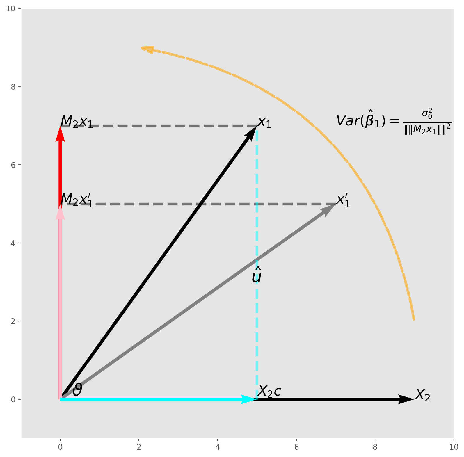

As we can see from the graph, if the length \(\|\boldsymbol{M}_2{x_1}\|\) is becoming longer means that the angle \(\vartheta\) is increasing on condition that \(\|x_1\|\) remain the same.

From linear algebra course, we know the formula

\[ \cos{\vartheta} = \frac{\boldsymbol{u}\cdot\boldsymbol{v}}{\|\boldsymbol{u}\|\|\boldsymbol{v}\|} \]

which is exactly the correlation coefficient. The larger the angle, the lower the correlation, i.e. smaller \(\cos{\vartheta}\).

In this example, if \(\boldsymbol{x}_1\) is highly correlated with \(\boldsymbol{X}_2\), then \(\vartheta\) must be relatively small, therefore \(\text{Var}(\hat{\beta})\) is relatively high. This is what we call multicollinearity in practice, though it is not really collinear, rather, approximately pointing to the same direction.

But remember this, multicollinearity always presents, but in a matter of degree, not yes or no.

We can also interpret the graph by using a standard regression model

\[ \boldsymbol{x}_1 = \boldsymbol{X}_2c + \hat{u} \]

where \(\hat{u} = \boldsymbol{M}_2\boldsymbol{x}_1\).

Comparing Precision of Estimators

If estimator \(\boldsymbol{\hat{\beta}}\) is more precise than \(\boldsymbol{\tilde{\beta}}\), the difference between them \[ \text{Var}(\boldsymbol{\tilde{\beta}})- \text{Var}(\boldsymbol{\hat{\beta}}) \] is a positive semidefinite matrix.

Also any linear combination of \(w^T\boldsymbol{\hat{\beta}}\) is also more efficient than \(w^T\boldsymbol{\tilde{\beta}}\), because \(\text{Var}(w^T\beta)=w^T\text{Var}(\beta)w\) \[ \boldsymbol{w}^{\top} \operatorname{Var}(\tilde{\boldsymbol{\beta}}) \boldsymbol{w}-\boldsymbol{w}^{\top} \operatorname{Var}(\hat{\boldsymbol{\beta}}) \boldsymbol{w}=\boldsymbol{w}^{\top}(\operatorname{Var}(\tilde{\boldsymbol{\beta}})-\operatorname{Var}(\hat{\boldsymbol{\beta}})) \boldsymbol{w}\geq0 \]

The Gauss-Markov Theorem

The principal result on efficiency of OLS estimator is called the Gauss-Markov Theorem. The informal way of stating this theorem is to say that \(\hat{\beta}\) is the best linear unbiased estimator (BLUE) .

Formally, if these two conditions are satisfied 1. \(E(\boldsymbol{u}|\boldsymbol{X})=\boldsymbol{0}\) 2. \(E(\boldsymbol{u}\boldsymbol{u}^T|\boldsymbol{X})=\sigma^2\mathbf{I}\) (homoskedasticity and uncorrelated \(u_t\))

OLS estimator is the BLUE.

The first condition holds because \[ E\left[\begin{array}{c} u_{1} \mid \boldsymbol{X} \\ u_{2} \mid \boldsymbol{X} \\ \vdots \\ u_{n} \mid \boldsymbol{X} \end{array}\right]=\left[\begin{array}{c} E\left(u_{1}\right) \\ E\left(u_{2}\right) \\ \vdots \\ E\left(u_{n}\right) \end{array}\right]=\left[\begin{array}{c} 0 \\ 0 \\ \vdots \\ 0 \end{array}\right] \]

The second condition can be shown \[ \begin{align} E\left(\boldsymbol{u u}^T \mid \boldsymbol{X}\right)&=E\left[\begin{array}{cccc} u_{1}^{2} \mid X & u_{1} u_{2} \mid X & \ldots & u_{1} u_{n} \mid X \\ u_{2} u_{1} \mid X & u_{2}^{2} \mid X & \ldots & u_{2} u_{n} \mid X \\ \vdots & \vdots & \vdots & \vdots \\ u_{n} u_{1} \mid X & u_{n} u_{2} \mid X & \ldots & u_{n}^{2} \mid X \end{array}\right]\\ &=\left[\begin{array}{cccc} E\left[u_{1}^{2} \mid X\right] & E\left[u_{1} u_{2} \mid X\right] & \ldots & E\left[u_{1} u_{n} \mid X\right] \\ E\left[u_{2} u_{1} \mid X\right] & E\left[u_{2}^{2} \mid X\right] & \ldots & E\left[u_{2} u_{n} \mid X\right] \\ \vdots & \vdots & \vdots & \vdots \\ E\left[u_{n} u_{1} \mid X\right] & E\left[u_{n} u_{2} \mid X\right] & \ldots & E\left[u_{n}^{2} \mid X\right] \end{array}\right]\\ &= \left[\begin{array}{cccc} \sigma^{2} & 0 & \ldots & 0 \\ 0 & \sigma^{2} & \ldots & 0 \\ \vdots & \vdots & \vdots & \vdots \\ 0 & 0 & \ldots & \sigma^{2} \end{array}\right] \end{align} \]

in the linear regression model, then OLS estimator \(\boldsymbol{\hat{\beta}}\) is more efficient than any other \(\boldsymbol{\tilde{\beta}}\), i.e. \(\text{Var}(\boldsymbol{\hat{\beta}}) - \text{Var}(\boldsymbol{\tilde{\beta}})\) is a positive semidefinite matrix.

Residuals and Disturbance Terms

We have discussed geometric and numerical properties of \(\hat{\boldsymbol{u}}\) in last chapter, here we will discuss the properties of \(\hat{\boldsymbol{u}}\).

One important insight from geometric view of OLS is \[ \|\boldsymbol{u}\| \geq \|\boldsymbol{\hat{u}}\| \] which is a direct deduction of \(\boldsymbol{\hat{u}}=\boldsymbol{M_Xu}\).

Expectation of Residuals

Consider two matrices \(\boldsymbol{A}_{n\times m}\) and \(\boldsymbol{B}_{m \times k}\), then the \(i^{th}\) row of \(\boldsymbol{AB}\) is the product of \(i^{th}\) row of \(\boldsymbol{A}\) and entire \(\boldsymbol{B}\), if we want to represent the \(t^{th}\) row of \(\boldsymbol{AB}\) we can use

\[ \boldsymbol{A}_t\boldsymbol{B} \]

where \(\boldsymbol{A}_t\) is the \(t^{th}\) row of \(\boldsymbol{A}\).

In general we can represent \(t^{th}\) row of a product of matrices by picking out the \(t^{th}\) row of the leftmost matrix.

Using this fact, we can denote the \(t^{th}\) residual as

\[ \hat{u}_t = \boldsymbol{M_X}\boldsymbol{u} = (\mathbf{I}-\boldsymbol{P_X})\boldsymbol{u} = u_t - \boldsymbol{X}_t(\boldsymbol{X}^T\boldsymbol{X})^{-1}\boldsymbol{X}^T\boldsymbol{u} \]

Although in Gauss-Markov Theorem, we assume the elements in error terms are independent, but this is not the case among residuals.

It is clear \(\boldsymbol{\hat{u}}\) is a linear combination of \(\boldsymbol{u}\) i.e. \(\boldsymbol{M_Xu}\), so the \(E(\boldsymbol{\hat{u}}) = \boldsymbol{0}\).

Variance of Residuals

Use the variance formula on \(\boldsymbol{\hat{u}}\)

\[\begin{align} \text{Var}(\boldsymbol{\hat{u}})&= \text{Var}(\boldsymbol{M_X}\boldsymbol{{u}}) = E[(\boldsymbol{M_X u}- E(\boldsymbol{M_X u}))(\boldsymbol{M_X u}- E(\boldsymbol{M_X u})^T)]\\ &= E(\boldsymbol{M_X}\boldsymbol{u}\boldsymbol{u}^T\boldsymbol{M_X}) = \boldsymbol{M_X}E(\boldsymbol{u}\boldsymbol{u}^T)\boldsymbol{M_X} = \boldsymbol{M_X}\text{Var}(\boldsymbol{u})\boldsymbol{M_X}\\ & = \boldsymbol{M_X}(\sigma_0^2\mathbf{I})\boldsymbol{M_X}\\ & = \sigma_0^2 \boldsymbol{M_X} \end{align}\]

Obviously, \(\boldsymbol{M_X}\) is not an identity matrix, which means that variances of \(\hat{u}_t\) might not be homoscedasticity, also \(E(u_tu_s)\neq 0\), i.e. the residuals are correlated.

We have denoted the \(t^{th}\) diagonal element of \(\boldsymbol{P_X}\) as \(h_t\), then the \(t^{th}\) diagonal element of \(\boldsymbol{M_X}\) is \(1-h_t\). In last chapter, we have shown that \(0 \leq h_t < 1\), hence \(0 \leq 1- h_t < 1\)

\[ \text{Var}(\hat{u}_t)<\sigma_0^2 \]

The variance of any residual from OLS is always smaller than variance of disturbance term, this feature determined by the mechanism of OLS algorithm.

Estimating the Variance of Error Terms

We do not observe the disturbance terms \(u_t\), neither does \(\sigma^2_0\). But we are able to estimate it by method of moments.

The simplest estimator of \(\sigma^2_0\) is

\[ \hat{\sigma}^2 = \frac{1}{n}\sum_{t=1}^n\hat{u}_t^2 \]

However we have shown \(\text{Var}(\hat{u}_t)<\sigma_0^2\), so \(\hat{\sigma}^2\) must be biased downward.

Before showing how to neutralize the bias, here is a side note about the trace of matrices.

The Trace of Matrices

The trace is the sum of the elements on the principal diagonal of a \(n\times n\) matrix, denoted \(\text{Tr}(\boldsymbol{A})\). And it can be a product of any two matrices \(\boldsymbol{A}_{n\times m} \boldsymbol{B}_{m \times n}\). But there is a convenient property called cyclic permutation.

\[ \text{Tr}(\boldsymbol{ABC}) = \text{Tr}(\boldsymbol{CAB}) = \text{Tr}(\boldsymbol{BCA}) \]

Because \(\boldsymbol{P_X}\) is a square matrix, we can use the formula onto \(\boldsymbol{P_X}\) and we can show that

\[ \text{Tr}(\boldsymbol{P_X})= \text{Tr}(\boldsymbol{X}(\boldsymbol{X}^T\boldsymbol{X})^{-1}\boldsymbol{X}^T) = \text{Tr}(\boldsymbol{X}^T\boldsymbol{X}(\boldsymbol{X}^T\boldsymbol{X})^{-1}) = \text{Tr}(\mathbf{I}_k) = k \]

Unbiased Estimator of Variance of Error Term

Let’s process with \(\hat{\sigma}^2\) by taking expectation

\[ E(\hat{\sigma}^2) = \frac{1}{n}\sum_{t=1}^nE(\hat{u}_t^2) \]

Use the fact that \(\text{Var}(\hat{u}_t) = E[(\hat{u}_t- E(\hat{u}_t))^2] = E[(\hat{u}_t)^2] = (1-h_t)\sigma_0^2\) and \(\text{Tr}(\mathbf{I}_k)=k\)

\[ \frac{1}{n}\sum_{t=1}^nE(\hat{u}_t^2) = \frac{1}{n}\sum_{t=1}^n(1-h_t)\sigma_0^2=\frac{n-k}{n}\sigma_0^2 \]

We have the unbiased estimator of \(\sigma^2\)

\[ s^2 = \frac{1}{n-k}\sum_{t=1}^nE(\hat{u}_t^2)= \frac{1}{n-k}\sum_{t=1}^n\hat{u}_t^2=\frac{\hat{u}^T\hat{u}}{n-k} \]

And now we can replace the \(\sigma_0^2\) in the \(\text{Var}(\boldsymbol{\hat{\beta}}) = \sigma_0^2(\boldsymbol{X^TX})^{-1}\), the square root of principal diagonal holds the standard error of \(\boldsymbol{\hat{\beta}}\).

\[ \widehat{\text{Var}}(\boldsymbol{\hat{\beta}}) = s^2(\boldsymbol{X^TX})^{-1} \]

Numerical Example of Residuals

Use the class or functions that I wrote in linregfunc.py, we can carry out a quick simulation comparing the modulus of residuals and disturbance term.

There are both class and functions in the linregfunc.py, we will choose the whatever the most convenient.

The moment when an object is instantiated, all the randomized data for OLS will be generated accordingly.

import linregfunc as lr

ols_obj = lr.OlsSim(100, 3, [6, 7, 8])

print("The moduduls of residual: {:.4f}".format(np.linalg.norm(ols_obj.resid)))
print("The moduduls of disturbance term: {:.4f}".format(np.linalg.norm(ols_obj.u)))

The moduduls of residual: 8.9888
The moduduls of disturbance term: 9.4675

It holds because theory guarantees \[ \text{Var}(\hat{u}_t)<\sigma_0^2 \]

However simulate this in a manner of distribution?

The function, which generates disturbance terms, follows a standard normal distribution, i.e. \(\sigma_0^2=1\). \(\hat{u}_t\) is a specific term of the residual vector, for instance to estimate the variance of \(\hat{u}_1\), we simulate the estimation process \(10000\) times, then calculate the variance from those \(10000\) \(\hat{u}_1\)’s.

Set sample size \(n=100\), create projection matrix \(\boldsymbol{M}\).

proj_matM = ols_obj.proj_mat_M()

We have create \(\boldsymbol{\beta} = [6, 7, 8]^T\). Now add a placeholder array for residuals.

resid_array = np.zeros([100, 1])

Generate \(10000\) vectors of residuals and stack them horizontally by specifying axis=1. gen_u is a function for generating disturbance term which is identical to the one used in the class OLS_Simu, for convenience of loops we use the function rather than method.

for i in range(10000):
    u = lr.gen_u(100)
    resid = proj_matM @ u
    resid_array = np.concatenate((resid_array, resid), axis=1)
resid_array = resid_array[:, 1:]

Because this is a sequence of simulations, the variance will be a frequency distribution rather than a single number. Here is the histogram, obviously the mean is less than \(1\) as we have expected.

fig, ax = plt.subplots(figsize=(10, 10))
ax.hist(np.var(resid_array, axis=0), bins=80)
ax.axvline(x=np.mean(np.var(resid_array, axis=0)), color="blue")
ax.set_title("Variance Distribution of Sampled Residuals")
plt.show()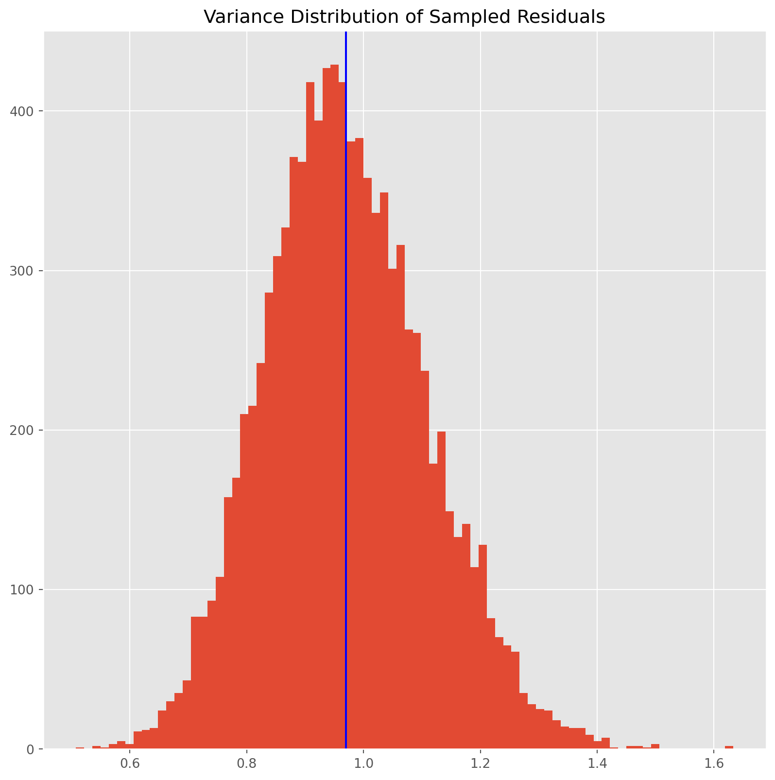

Standard Errors Simulation

Here we simply show a numerical example of covariance matrix and the square root of its principal diagonal which holds the standard errors of \(\hat{\boldsymbol{\beta}}\).

ols_obj = lr.OlsSim(100, 4, [6, 7, 8, 9])
cov_betahat, cov_betahat_diag = ols_obj.cov_beta_hat()

np.sqrt(cov_betahat_diag)

array([0.09536819, 0.09189692, 0.103185  , 0.09876602])

Compare with statsmodels results.

ols_obj_fit = sm.OLS(ols_obj.y, ols_obj.X).fit()
print(ols_obj_fit.bse)

[0.09536819 0.09189692 0.103185   0.09876602]

Results are exactly the same.